Index Function In Excel-1
INDEX
This function picks a value from a range of data by looking down a specified number of rows and then across a specified number of columns.
यह फंक्शन एक डाटा के दिए गए range से नीचे की ओर से number of rows और फिर दिए गए columns से डाटा उठाता है.
Syntax
There are various forms of syntax for this function.
इस फंक्शन के लिए अनेक प्रकार का syntax है.
Syntax 1
=INDEX(RangeToLookIn, Coordinate)
This is used when the RangeToLookIn is either a single column or row.
इसे हम तब प्रयोग करते हैं, जब data, single row या column में हो.
The Coordinate indicates how far down or across to look when picking the data from the range.
Coordinate बताता है की data Pick करते समय नीचे या तिरछे कितना जाना है.
Both of the examples given below use the same syntax, but the Co-ordinate refers to a row when the range is vertical and a column when the range is horizontal.
नीचे दिए दोनों example में हम same syntax का प्रयोग करते हैं, लेकिन coordinate row को दर्शाता है जब data vertical है, और coordinate column को दर्शाता है जब डाटा horizontal हो.
Example:-1
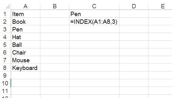
Here we have used index function with vertical data.
यहाँ हमने vertical डाटा के साथ index function का प्रयोग किया है.
Here we have picked 3rd item from data range A1:A8, which is pen.
यहाँ हम A1:A8 डाटा रेंज से तीसरा आइटम उठाया है, जो कि pen है.
Example:-2
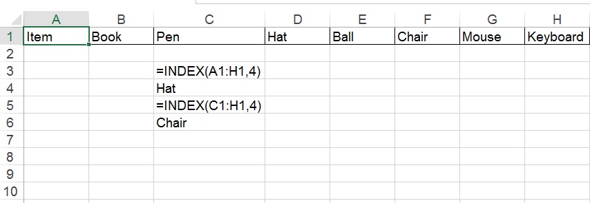
Here we have used index function with horizontal data.
यहाँ हमने horizontal डाटा के साथ index function का प्रयोग किया है.
Here we have picked 4th item from data range A1:H1, which is Hat.
यहाँ हम A1:H1 डाटा रेंज से 4th item उठाया है, जो कि hat है.
We will update more example of index.
हम Index का और उदाहरण प्रदान करेंगे।
9:09 am
thank you to share it with me ..