Index Function In Excel-2
Index
With the help of INDEX function in excel we get value from a table or range on the intersection of a row and column position within the table or range. The first row in the table is row 1 and the first column in the table is column 1.
एक्सेल मं हम Index फंक्शन की मदद से table या range से हम row और columne के कटाव का value प्राप्त करते हैं. पहला row table में row 1 और पहला column table में column 1
Row 1 means first row of the table and column 1 means first column of the table.
Row 1 मतलब table का पहला row और column 1 मतलब table का पहला column
INDEX function can be used in excel when you want to fetch the value from a tabular data and you have the row number and column number of the data point.
Index function का उपयोग कर एक्सेल में हम data से value निकालते हैं, जब हमारे पास row और column नंबर हो.
Syntax
INDEX(array, row_num, [column_num])
INDEX(Data_Range, row_number, column_number )
In below table I want to salary of John.
नीचे के टेबल से मैं जॉन का सैलरी निकलना चाहता हूँ.
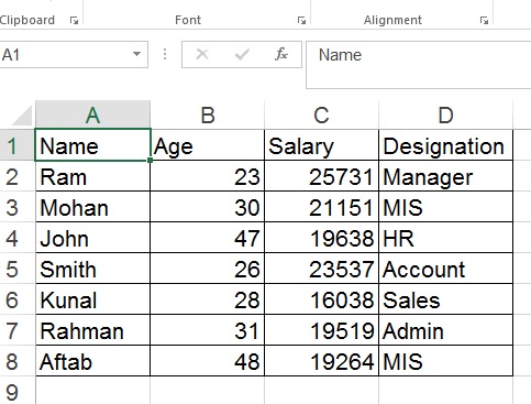
In the range A1:D8, John at 4th row and Salary at 3rd Column. The salary amount of john will be intersection of 4th row & 3rd Column.
रेंज A1:A8 में, John 4th row मैं है और salary 3rd column में है. जॉन का salary amount 4th row और 3rd column कटाव होगा.
For this we have to type formula =INDEX(A1:D8,4,3), It will pick value 19638 from range A1:D8, which is intersection of 4th row, 3rd column.
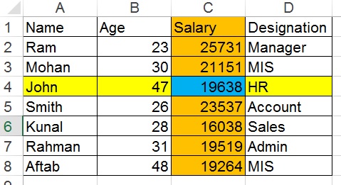
इसके लिए हमें =INDEX(A1:D8,4,3) formula टाइप करना होगा. यह 19638, range A1:D8 से उठाएगा, जो कि 4th row और 3rd column का कटाव है.