Indirect Function In Excel -1
We use Indirect function in excel to converts a plain piece of text which looks like a cell address into a usable cell reference.
एक्सेल में Indirect Function का प्रयोग कर हम Cell Address की तरह दिखने वाले Plain text को usable cell referent में convert करते हैं.
The address can be either on the same worksheet or on a different worksheet.
Address उसी sheet पर हो सकता है या फिर दूसरे sheet पर.
Syntax
INDIRECT(ref_text, [a1])
INDIRECT Function Arguments
The INDIRECT function has two arguments: INDIRECT(ref_text,a1)
If ref_text is not a valid cell reference, INDIRECT returns the #REF! error value.
अगर ref text valid cell नहीं है तो Indirect function #REF! error देगा.
[a1]: Optional. A logical value that specifies what type of reference is contained in the cell ref_text.
यह ऑप्शनल है, एक लॉजिकल वैल्यू जो निर्दिष्ट करता है कि सेल Ref_text में किस प्रकार का reference है।
If a1 is TRUE or omitted, ref_text is interpreted as an A1-style reference.
यदि a1 TRUE है या खाली है, तो ref_text को A1-style reference. को represent करता है.
If a1 is FALSE, ref_text is interpreted as an R1C1-style reference
यदि a1 false है, तो ref_text को R1C1-style reference. को represent करता है.
Example:-1
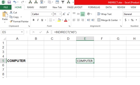
A5 cell has a value COMPUTER
A5 cell में कंप्यूटर लिखा है.
If we type FORMULA =INDIRECT(“A5”) in cell E9, then output will be COMPUTER
अगर हम E9 cell में =INDIRECT(“A5”) टाइप करते है, तो output COMPUTER आएगा.
Example:-2
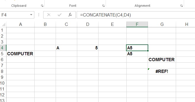
Here C4 Cell has a value A and D4 cell has a value 5. I concatenate both value in F4 cell with formula =CONCATENATE(C4,D4) OR =C4&D4, output will be shown A5, then type formula =INDIRECT(F4) in G6 cell.
यहाँ C4 cell में A value है और D4 cell में 5 value है. मैंने दोनों value को concatenate कर दिया F4 cell में =CONCATENATE(C4,D4) OR =C4&D4 formula से, तो output A5 आ गया. तब मैं G6 cell में =INDIRECT(F4) formula टाइप किया.
The formula located to cell F4, fetches its value – text string A5, converts it into a cell reference, which picks value from A5 cell and returns its value, which is COMPUTER
F4 cell में जो फार्मूला है ,वो A5 को string की तरह value को pick करता है, इसे cell reference, मैं परिवर्तित करता है, जो A5 cell से value को उठाता है और आउटपुट computer आ जाता है.
If we type =INDIRECT(F4,0), then excel will give error, because 0 used for R1C1-style reference, but here f4, A1 Style reference
अगर हम =INDIRECT(F4,0), फार्मूला यहाँ टाइप करते हैं तो एक्सेल error देगा, क्योंकि 0 का प्रयोग R1C1-style रिफरेन्स में होता है, लेकिन यहाँ F4, A1 Style reference है.
Example:-3
FOR R1C1 references:
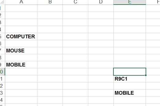
I have typed R9C1 in E11 cell, where R represent row, means row 9, and C represent column, means column 1
Now typed =INDIRECT(E11,0) in cell E13, here 0 or false in the 2nd argument indicates that the referred value (E11) should be treated like a R1C1 cell reference.
INDIRECT function interprets the value in cell E11 (R9C1) as a reference to the cell at the conjunction of row 9 and column 1, which is cell A9.
Example:-4
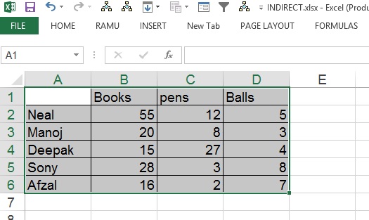
Here is a small data, I have made below 3 named ranges
यहाँ एक डाटा है, मैंने ३ named range नीचे लिखे नाम और रेंज से बनाया है.
Books – B2:B6
Pens – C2:C6
Balls – D2:D6
Now I will type books, pens or balls one by one in F1 cell and type formula =SUM(INDIRECT(F1)) in G1 cell.
अब मैं books, pens और balls बारी बारी से F1 cell में टाइप करुगा, और G1 cell में =SUM(INDIRECT(F1)) फार्मूला type करता हूँ,

It will give sum of that value which is being typed in F1 cell
यह हमें F1 cell में टाइप किये जा रहे value का sum देगा.