Match With Index In Excel
Use of Match Function With Index
Match Function के साथ Index फंक्शन का प्रयोग
The INDEX MATCH formula is the combination of two functions in Excel: INDEX and MATCH.
INDEX MATCH formula Excel में Index और Match दो Functions का संयोजन है।
=INDEX() returns the value of a cell in a table based on the column and row number.
Column और Row की संख्या के आधार पर तालिका में cell का Value लौटाता है।
=MATCH() returns the position of a cell in a row or column.
MATCH () row या column में cell की स्थान बताता है।
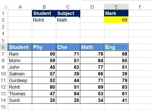
We have made drop down in B2 cell for student name and in C2 cell for Subject name.
हमने Student नाम के लिए B2 cell में और Subject नाम के लिए C2 Cell में Drop Down बनाया है।
From above table I want to know any subject mark of any student.
ऊपर की तालिका से मैं किसी भी छात्र के किसी भी विषय का Mark जानना चाहता हूं।
I want result in E2 cell, from drop down which student & subject will be selected, respective result will be shown in E2 cell.
मुझे E2 Cell में परिणाम चाहिए, ड्रॉप डाउन से जो छात्र और विषय का चयन किया जाएगा, उसका Mark E2 सेल में दिखाया जाएगा।
For example if we choose Rohit from B2 Cell, and subject name Math from C2 Cell, then Rohit’s Math mark will be shown in E2 cell, which is 69.
उदाहरण के लिए यदि हम B2 सेल से रोहित को चुनते हैं, और C2 सेल से विषय का नाम Math लेते हैं, तो रोहित का गणित का Mark E2 सेल में दिखेगा जो कि 69 है।
For that we need to find out what is the position of that student in range A6:A14, whose mark we are searching in this table and need to find out what is the position of that subject in range AE:A6.
इसके लिए हमें यह पता करना होगा की Range A6:A14 में उस स्टूडेंट का स्थान कौन सा है, जिसका Mark हम इस टेबल में खोज रहें है और हमें यह पता करना होगा की उस Subject का पोजीशन रेंज A6:E6 में क्या है.
We have to type formula for Student position in G6 cell, =MATCH(B2,A6:A14,0)
स्टूडेंट का position प्राप्त करने के लिए हमें G6 Cell में =MATCH(B2,A6:A14,0) टाइप करना होगा.
It will give position of student name which we have selected in B2 cell.
यह हमें उस Student का position देगा जो हमने B2 Cell में Select किया है.
We have to type formula for Subject position in G7 cell, =MATCH(C2,A6:E6,0)
Subject का position प्राप्त करने के लिए G7 Cell में =MATCH(C2,A6:E6,0) टाइप करना होगा.
It will give position of Subject name which we have select in C2 cell.
यह हमें उस Subject का Position देगा जो हमने C2 Cell में Select किया है.
In E2 Cell we will type formula =INDEX(A6:E14,G6,G7) and now we have to paste formula which we used in G6 cell for find out name position.
E2 Cell में हमें =INDEX(A6:E14,G6,G7) इस फार्मूला को टाइप करना होगा और अब हमें G6 Cell का फार्मूला यहाँ G6 के बदले पेस्ट करना होगा.
=INDEX(A6:E14,MATCH(B2,A6:A14,0),G7)
same need to paste formula which we used in G7 cell for find out subject position.
उसी तरह G7 कर Formula G7 के बदले paste करना होगा.
Finally this formula will be looked like below.
अंत में यह Formula नीचे जैसा दिखेगा।
=INDEX(A6:E14,MATCH(B2,A6:A14,0),MATCH(C2,A6:E6,0))
Now it became complete formula. We can now find out any student’s any subject mark with using drop down list from B2 & C2 Cell.
अब यह complete formula बन गया है। अब हम B2 और C2 सेल से ड्रॉप डाउन List का उपयोग करके किसी भी छात्र के किसी भी विषय के Mark का पता लगा सकते हैं।
10:12 am
Sir i just want to learn vba but how it works why we use it why from begging pls help me to learn vba
10:44 pm
https://www.youtube.com/watch?v=WH0ex_u0lcw
VBA MACRO INTRODUCTION
10:45 pm
VBA MACRO CLASS 1