Match_Function
MATCH Function in Excel
एक्सेल में मैच फंक्शन का प्रयोग
With the help of match function we find out position of a lookup value in a row or column. It does not return the value. MATCH supports approximate and exact matching, and wildcards (* ?) for partial matches. We often use match with Index and Vlookup for getting data. It can be used with text and numbers. This function looks for an item in a list and shows its position.
Match फंक्शन की मदद से हम lookup value का position row और column से प्राप्त करते हैं. यह value return नहीं करता है. MATCH अनुमानित और ठीक ठीक मिलान का समर्थन करता है. और wildcards(*) से partial मैच करता है. हम लोग अक्सर match का प्रयोग Index और lookup के साथ Data प्राप्त करने के लिए करते है. यह Function लिस्ट में एक Value को खोजता है और उसका पोजीशन बताता है.
———-
Syntax
=MATCH (lookup_value, lookup_array, [match_type])
=MATCH(WhatToLookFor, WhereToLook ,TypeOfMatch)
lookup_value is the value you tell the match function to lookup
एक विशिष्ट पहचानकर्ता वाला सेल(Cell)
lookup_array is the list that you look an item up in
आपके द्वारा खोज रहे cell ka range
[match_type] tells the MATCH what sort of lookup to do:
बताता है कि किस प्रकार का लुकअप करना है:
The TypeOfMatch either 0, 1 or -1.
Example:- Use of Match type 0

ऊपर के इमेज में, B3 से B10 तक कुछ डाटा है. मैच फंक्शन का प्रयोग कर, हम D का पोजीशन इस रेंज में पता कर रहे है. इसके लिए हमें =match(“D”,B3:B10,0) फार्मूला टाइप करना होगा.
यह 4 return करेगा, मतलब D value range B3:B10 में 4th पोजीशन पर है. अगर हम Q का position इस range में पता करेंगे तो यह #N/A का error show करेगा. इसका मतलब है कि Q इस range में नहीं है.
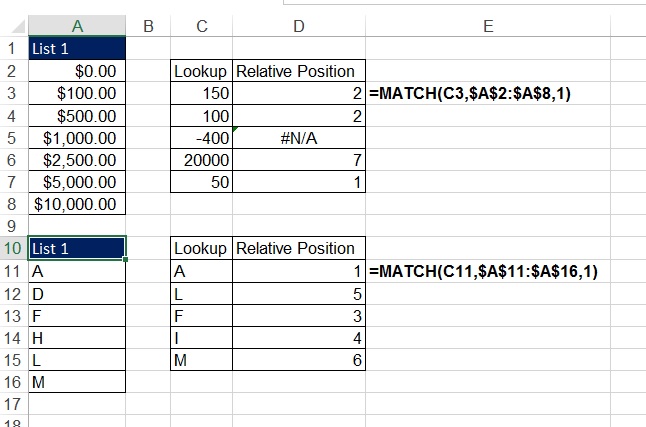
Example:- Use of match type 1
If match_type is 1, MATCH finds the largest value that is less than or equal to lookup_value. The lookup_array must be sorted in ascending order.
अगर मैच type 1 है, तो मैच सबसे बड़े value को खोजता है जो lookup_value के बराबर या कम है. Lookup_array आरोही क्रम में क्रमबद्ध होना चाहिए।
Using 1 will look for an exact match, or the next lowest number if no exact match exists.
1 का प्रयोग करने पर, lookup value पहले exact match तलाश करेगा, अगर exact match नहीं मिला तो, यह अगला न्यूनतम संख्या का पोजीशन बताएगा.
If there is no match or next lowest number the error #N/A is shown.
अगर exact मैच या अगला न्यूनतम संख्या नहीं मिला तो यह error #N/A शो करेगा.
The lookup_array must be sorted in ascending order for this to work correctly.
इसे सही तरीके से काम करने के लिए lookup_array का आरोही क्रम में अवश्य क्रमबद्ध किया होना चाहिए।.
Example:- Use of match type -1
If match_type is -1, MATCH finds the smallest value that is greater than or equal to lookup_value. The lookup_array must be sorted in descending order.
अगर मैच type -1 है, तो मैच सबसे छोटा value को खोजता है जो lookup_value के बराबर या अधिक है. Lookup_array घटते क्रम में क्रमबद्ध होना चाहिए।
Using -1 will look for an exact match, or the next largest number if no exact match exists.
-1 का प्रयोग करने पर, lookup value पहले exact match तलाश करेगा, अगर exact match नहीं मिला तो, यह अगला बड़ा संख्या का पोजीशन बताएगा.
If there is no match or next largest number the error #N/A is shown.
अगर exact मैच या अगला बड़ा संख्या नहीं मिला तो यह error #N/A शो करेगा.
The lookup_array must be sorted in descending order for this to work correctly.
इसे सही तरीके से काम करने के लिए lookup_array का घटते क्रम में अवश्य क्रमबद्ध
किया होना चाहिए।

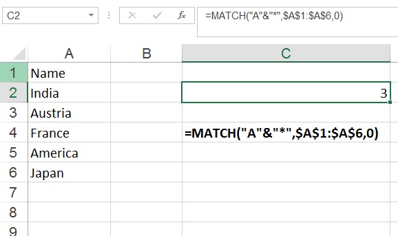
Example:- Use match with Wildcard
Sometimes it happens that we want not to match entire string, but only some characters or some part of the string. Wildcards can be used with match_type 0 only.
कभी कभी ऐसा होता है कि हम पूरा string न match करके कुछ characters या string का कुछ हिस्सा मैच करे. वाइल्डकार्ड का उपयोग केवल match_type 0 के साथ किया जा सकता है।